4.3Nondeterministic Finite Automata

The finite automata we have seen so far are deterministic finite automata (DFA): given the current state and the next input symbol, there is exactly one state that a finite automaton can move to. In this section, we introduce nondeterministic finite automata (NFA), which have two additional features:

1. An NFA’s state transition function takes as input the current state and the next input symbol, and is allowed to return, not just one state, but a subset of states.

2. An NFA is also allowed to make transitions without consuming the next input symbol. These are called $ε$-transitions as it is as if the next input symbol is the empty string.

We will introduce these two features one by one.

4.3.1Transition to more than one state¶

Let $N$ be an NFA without $ε$-transitions. Consider a string $w = v_1 v_2 \cdots v_n$ where each $v_i$ is an input symbol from $\Sigma$. The NFA processes $w$ as follows. We use $S_i$ to denote the set of states the NFA is in after processing $v_1\cdots v_i$.

1. Start at the start state: $S_0 = \{q_0\}$.

2. For each input symbol $v_i$ (starting from $v_1$): define $S_i$ to consist of states $r$ such that there exists $q \in S_{i-1}$ and $r = \delta(q,v_i)$.

3. After all input symbols have been processed, it accepts the string if $S_n$ contains an accepting state, and rejects it otherwise.

We can also view the NFA as having several possible state transition sequences of the form

where $r_i \in \delta(r_{i-1}, v_i)$ for each $i$ ranging from 1 to $n$. Note that since $\delta(r_{i-1},v_i)$ can be a set of more than one state, there can be several possible state transition sequences, and so there may be several resulting states. We denote by $Q(w)$ the set of resulting states.

The high level interpretation is as follows: Suppose the NFA $N$ is at state $q$, the next input symbol is 0, and $\delta(q,0) = S$ for some set of states $S$. Then, $N$ simultaneously transitions to all of them, in parallel. Each of these parallel “threads” then process the input independently of each other. Metaphorically, the universe is “split” into $k$ parallel universes, where $k$ is the size of $S$. The NFA accepts the string iff it ends up in an accepting state in one of the universes.

Computation tree¶

Similar to DFAs, we can define a computation path to be a sequence of state transitions followed by $N$ while processing $w$. We say that the path is accepting path if it ends in an accepting state and rejecting otherwise. Thus, an NFA accepts a string $w$ iff there exists an accepting computation path.

Observe that with DFAs, we have a single computation path for each input string. NFAs on the other hand, can have multiple computation paths. Consider the following NFA.

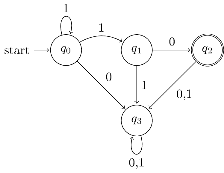
On input 110, it has 3 possible state transition sequences, each corresponding to a computation path.

We can in turn represent these paths using a tree, which we call a computation tree.

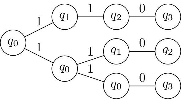
In this example, the string 110 is accepted by the NFA as there is one computation path (the one in the middle) ending in an accepting state.

4.3.2epsilon-transitions¶

An NFA with $ε$-transitions is one where instead of consuming the next input symbol and processing it using the transition function, the NFA can instead choose to follow an $ε$-transition which is a transition that does not consume the next input symbol.

Thus, in the state transition diagram, there may be edges that are labeled with $\epsilon$ instead of a symbol from $\Sigma$. Suppose the NFA $N$ is at state $q$, the next input symbol is 0, and $\delta(q,\epsilon) = S$ for some set of states $S$. Then, $N$ can immediately transition simultaneously to the states in $S$.

Let $N$ be an NFA. Consider a string $w = v_1 v_2 \cdots v_n$ where each $v_i \in \Sigma \cup \{\epsilon\}$. A state $q$ is a resulting state of $N$ after processing $w$ iff there exists a sequence of state transitions:

where $r_0 = q_0$, and $r_i \in \delta(r_{i-1}, v_i)$. Note that there may be several resulting states. We denote by $Q(w)$ the set of resulting states.

The definition of acceptance is the same as for NFAs without $ε$-transitions (Definition 2).

Computation tree¶

Consider the following NFA.

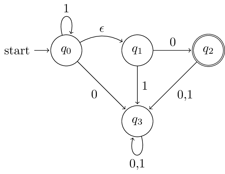
On input 10, it has 3 possible state transition sequences, each again corresponding to a computation path.

Here is its computation tree. Observe that for every root-to-leaf path, concatenating the symbols on the path gives us 10.

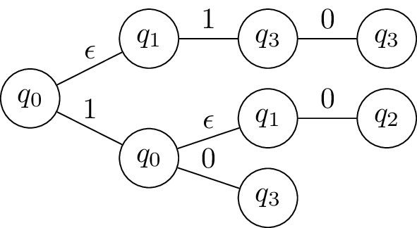
In this example, the string 10 is accepted by the NFA as there is one computation path (the one in the middle) ending in an accepting state.